End-to-end Machine Learning System

Supply Chain Demand Forecasting & Inventory Optimization

A production-grade ML pipeline that forecasts daily sales for 3,049 retail SKUs, translates those forecasts into purchasing decisions, and serves everything through a REST API and interactive dashboard — built on the Walmart M5 competition dataset.

LightGBM Time Series Quantile Regression Inventory Optimization FastAPI Optuna HPO Streamlit Python
3,049
SKUs modeled
29%
RMSE vs baseline
93.5%
Series LGB wins
0.911
WRMSSE (28-day)
3.1%
Walk-forward CV

Two costs that pull in opposite directions

Retailers carry inventory under fundamental uncertainty about future demand. Get it wrong in either direction and you pay:

Overstock
Units sit on shelves, capital is locked, markdowns erode margin
Stockout
Empty shelf, lost sale, potential permanent customer loss
3,049
Simultaneous decisions
One store, one day — each SKU needs its own forecast and order trigger
<1s
Computation time
Full inventory params for all 3,049 items in under a second

Getting the balance right requires knowing, as accurately as possible, how much of each product will sell over the next four weeks — and how uncertain that estimate is. This project builds the full system: from raw sales history to a live API that answers both questions on demand.

Walmart M5: one of the hardest public forecasting benchmarks

The M5 Forecasting Competition dataset contains hierarchical daily unit sales from Walmart stores across three U.S. states. The pipeline is demonstrated on CA_1 (California, Store 1) with the option to scale to all 10 stores in parallel.

DimensionValue
StoreCA_1 — Walmart California, Store 1
SKUs modeled3,049 unique items
History per item~1,941 daily observations (2011–2016)
Total rows (long format)~5.9 million
CategoriesFOODS, HOBBIES, HOUSEHOLD
Departments7 (FOODS_1/2/3, HOBBIES_1/2, HOUSEHOLD_1/2)
External signalsCalendar events, SNAP food-stamp flags, daily sell price

Raw data arrives in wide format — one column per day, one row per item. The pipeline immediately melts it to long format (item × date rows), merges the calendar and price tables, and applies dtype optimization (categoricals, float32 lags) to keep memory under 2 GB.

Aggregate Sales Trend, 2011–2016

Aggregate daily sales trend with 28-day rolling mean
Blue bars: daily total units sold across all 3,049 items. Red line: 28-day rolling mean. Sales grew roughly 25–30% over the period. The series is non-stationary — the mean drifts upward — so a model cannot simply assume the future looks like the historical average. Recurring dips are store closures; spikes are promotional events.

Seasonality Patterns

Sales by day of week and month of year
Left: Day-of-week distribution. Monday shows higher variance; Friday–Sunday have tighter, slightly higher medians — weekend shopping is more predictable and modestly higher volume. Right: Monthly averages. Summer (Jun–Aug) shows a small consistent uplift (~8% peak-to-trough). Weekly and event-driven seasonality dominate over annual cycles for this store.

Event & SNAP Impact

Sales uplift on event days and SNAP days
SNAP days (federal food-stamp disbursement) show a statistically measurable +5.3% mean uplift (3.75 vs 3.56 units per non-zero transaction). Calendar events (sporting events, cultural holidays) show no aggregate lift — their impact varies by specific SKU rather than lifting the whole store. SNAP flags are high-value model features; event flags are included but low-importance at store level.

One global LightGBM model for 3,049 SKUs

Rather than fitting 3,049 separate models, the pipeline trains a single global LightGBM model that ingests all items simultaneously. Each row is one (item, date) pair — the model learns what distinguishes items and time periods from each other.

The global approach has three advantages over per-series models:

Objective Function: Tweedie Regression

LightGBM is configured with Tweedie loss rather than squared-error. Retail sales are zero-inflated and right-skewed — most (item, day) pairs sell 0–2 units, but occasionally an item sells 20+. Squared-error gets dominated by those outliers. Tweedie is the proper distribution for compound Poisson count data.

The Tweedie variance power p = 1.231 was found by Optuna (between Poisson p=1 and Gamma p=2), reflecting moderate overdispersion.

Feature Engineering

GroupFeaturesWhat it encodes
Lag featureslag_7, lag_14, lag_28, lag_35Sales from 1/2/4/5 weeks ago — weekly seasonality signal
Rolling meansroll_mean_7/14/28Recent demand level — the model's "memory" of how fast this item sells
Rolling stdroll_std_7/14/28Demand volatility — high-std items need more safety stock
Price featuressell_price, price_rel_store_cat, price_pct_4wAbsolute price, price vs. category peers, recent price change
Calendarwday_sin/cos, week_sin/cos, month, yearCyclical encodings avoid discontinuity at week/year boundaries
Eventshas_event, snapBinary flags for known demand shocks
Identityitem_id, dept_id, cat_idCategorical embeddings — model learns item-specific baselines

Feature Importance

LightGBM feature importance by gain and split count
Gain (left) — average reduction in loss per split. roll_mean_14 alone contributes ~45% of total gain. The model primarily answers "how much did this item sell in the last 2 weeks?" before anything else. Split count (right) — how many times a feature appears in the ensemble. item_id appears 70,000+ times — the model makes fine-grained item-level adjustments throughout every tree, even though each individual adjustment is small. Insight: the dominant features are endogenous (derived from past sales), not exogenous. The model is a sophisticated autoregressive smoother. Price and events matter at the margin.

Hyperparameter Optimization with Optuna

Rather than grid search, the pipeline uses Optuna TPE (Tree-structured Parzen Estimator) — a Bayesian optimization algorithm that builds a probabilistic model of the loss surface and proposes new configurations intelligently. 20 trials over 7 hyperparameters.

Optuna tuning history showing convergence to best RMSE
Each dot is one trial. The red line tracks the running best RMSE. Optuna converged on a promising region by trial 11. Best: RMSE = 2.018 at trial 15 with learning rate 0.0147, 223 leaves, L2 regularization 0.573.

Results: LightGBM vs Naive Seasonal Baseline

The benchmark is Naive Seasonal — which predicts that any day's sales will equal the same weekday from 4 weeks ago. This is a strong baseline for retail data; beating it requires genuinely capturing patterns the calendar can't explain.

Bar chart: LightGBM vs Naive Seasonal on RMSE, MAE, MASE
All three metrics favor LightGBM. Lower is better.

LightGBM (Global Model)

RMSE1.396
MAE1.069
MASE1.383
Win rate vs naive93.5%

Naive Seasonal (Baseline)

RMSE1.969
MAE1.412
MASE1.653
Improvement

RMSE — average forecast error in units, with larger errors penalized quadratically.   MAE — average absolute error in units.   MASE — MAE scaled by the naive baseline on training data; values near 1 mean the model performs like naive on training but outperforms on held-out validation — the expected pattern for a model that generalizes while per-item naive baselines overfit historical noise.

28-day recursive forecasting with uncertainty bands

Prediction Intervals (Phase 4)

A point forecast alone is incomplete for inventory decisions. Three separate LightGBM models are trained with quantile (pinball) loss at the 10th, 50th, and 90th percentiles to bound uncertainty.

P10
Lower bound
90% chance actual sales exceed this
P50
Median
50th percentile — not the mean
P90
Upper bound
90% chance actual sales fall below this
Prediction interval coverage for sample series
Each panel: actual sales (black line) vs P10–P90 shaded band over the validation period. Coverage annotations show what fraction of actual values fell inside the band. Aggregate 80% interval coverage: 83.4% — slightly above the nominal 80% target, meaning intervals are mildly conservative (slightly wide). For inventory, this is the preferred direction: underestimating uncertainty is riskier than overestimating it. Mean interval width: 3.14 units.

Recursive 28-Day Forecast (Phase 5)

In operations, you need the full 4-week horizon at once to calculate how much to order today — not just tomorrow's number. Recursive forecasting delivers this by treating each day's prediction as the input to the next.

The recursive challenge: the model was trained on features like lag_7 (sales 7 days ago). On forecast day 8, "7 days ago" is itself a predicted value. The pipeline handles this with a rolling buffer — each step appends its own output and recomputes all lag/rolling features before predicting the next.

Recursive 28-day forecasts for sample items
Six sample items across all three categories. Blue bars: actual sales. Black dashed: recursive point forecast. Green band: P10–P90 interval from Phase 4. Items with regular weekly rhythm (FOODS_3) show the model tracking it cleanly. Sparse items (HOBBIES) get near-zero predictions with appropriate wide uncertainty. Intervals widen correctly for volatile series.

WRMSSE — The M5 Competition Metric

Weighted Root Mean Squared Scaled Error is the official M5 metric. It measures forecast accuracy, normalized by each item's historical variance, then weighted by that item's revenue contribution. A score of 1.0 means the model performs identically to the naïve seasonal baseline. Lower is better.

0.877
WRMSSE — One-step
Validation set, predict one day at a time
0.911
WRMSSE — Recursive 28d
Full 28-day horizon, compounding predictions
+3.9%
Recursive degradation
Error from compounding predictions — small, indicating stable features

Translating forecasts into purchasing decisions

A forecast that lives only in a CSV is not useful. Phase 6 converts each item's demand forecast and uncertainty estimate into three concrete purchasing parameters using the continuous-review inventory model — the same framework used by major retailers worldwide.

Safety Stock

Buffer inventory held to absorb demand uncertainty during the replenishment lead time. Higher uncertainty and longer lead times both require more buffer.

SS = z(SL) × σ_daily × √(lead_time)

z(SL) — z-score for target service level (1.645 at 95% SL)
σ_daily — daily demand std dev, derived from P10/P90 quantile spread
√(lead_time) — uncertainty compounds as square root of time

σ is derived from Phase 4's quantile spread: for a normal distribution, P90 − P10 ≈ 2.563 × σ. The quantile models do double duty — prediction intervals and volatility estimates for inventory.

Reorder Point

The inventory level at which a replenishment order is triggered. Designed so that, in the average demand scenario, inventory won't reach zero before the order arrives.

ROP = (mean_daily_demand × lead_time) + safety_stock

Economic Order Quantity

How much to order each time. Balances the cost of ordering frequently (fixed $50 per order) against the cost of holding large quantities (capital tied up, warehouse space).

EOQ = √(2 × D_annual × order_cost / holding_cost_per_unit)

D_annual — annual demand (daily mean × 365)
order_cost — fixed cost to place one order ($50 default)
holding_cost — cost of holding one unit per year (rate × unit_cost)

Inventory Overview — CA_1 (3,049 items)

Inventory optimization overview: scatter and top-20 bar chart
Left (log-log scatter): Each dot is one SKU. Mean daily demand vs safety stock. The tight linear relationship confirms model consistency — higher-demand items get proportionally higher safety stock. Bubble color encodes safety stock magnitude; the red dots in the upper right are high-volume items needing 80–100+ units of buffer. Right: Top 20 items by safety stock. FOODS_3_090 (highest priority): 104 units of safety stock (blue) plus 387 units of lead-time demand coverage (orange) — a total reorder point of 490 units. These are the items where a stockout is most expensive.

Store-Level Summary

MetricMeanMedianMax
Mean daily demand (units)1.520.7955.2
Safety stock (units)5.143.70103.8
Reorder point (units)15.769.20490.3
EOQ (units per order)445.5378.93,174.5
Days of supply in safety stock5.164.6017.1

The median item needs fewer than 4 units of safety stock and triggers an order at 9 units on hand — appropriate for slow-moving SKUs. The top-volume items (ROP = 490) require daily monitoring and represent an operationally different challenge.

Walk-forward validation: proving the model generalizes

Evaluating on a single held-out period can be misleading — maybe the model got lucky on that particular window. Walk-forward (rolling-origin) validation tests the model on four consecutive future windows, retraining from scratch at each origin.

──── Training data ────┤ Val (28d) │ ──── Training (extended) ──┤ Val (28d) │ ──── Training (further) ──────┤ Val (28d) │ ← repeat 4×

This simulates production: the model is retrained periodically as new data arrives, then evaluated on the next month it has never seen.

Walk-forward RMSE and MAE stability across 4 windows
LightGBM (green, solid) maintains a 27–30% RMSE reduction over Naive Seasonal (blue dashed) across all four validation windows. The shaded region is the performance gap — it stays wide and consistent. There is no window where the model struggles while the baseline excels. RMSE CV = 3.1% across windows — well below the 10% threshold for "stable." The model's advantage is not time-specific.
WindowValidation PeriodLightGBM RMSENaive RMSEReductionLGB Wins (%)
W1Feb 20161.3121.804−27%86.7%
W2Mar 20161.3101.840−29%87.4%
W3Apr 20161.3501.923−30%89.2%
W4May 20161.4001.969−29%93.6%

The slight upward drift in RMSE in later windows is matched by the baseline's own drift — the relative improvement stays flat. This means signal-to-noise in the data is stable; the model is not degrading.

REST API + Interactive Dashboard

The batch pipeline writes Parquet outputs once (or on schedule). The FastAPI server is the low-latency serving layer on top: reads outputs, caches DataFrames in memory with a 1-hour TTL, and answers queries in milliseconds.

MethodPathPurposeLatency
GET /health Liveness check — returns available stores and cache status <1 ms
GET /stores Lists all stores with completed pipeline outputs <1 ms
GET /stores/{store}/items Lists item IDs, filterable by category or department <5 ms
GET /forecast/{store}/{item_id} 28-day point + quantile forecast (pre-computed from Parquet) <5 ms
POST /inventory Live inventory params — any lead time or service level <1 ms
GET /metrics/{store} Store-level WRMSSE and walk-forward CV <2 ms

Design note: /forecast reads from Parquet — not from the live model. This means sub-millisecond response times at the cost of freshness (refresh by re-running Phase 5). /inventory computes on-the-fly, letting users query any lead time or service level without re-running Phase 6.

Example: Forecast Response

GET /forecast/CA_1/FOODS_1_001_CA_1_evaluation

{
  "store":    "CA_1",
  "item_id":  "FOODS_1_001_CA_1_evaluation",
  "n_days":   28,
  "forecasts": [
    {
      "date":         "2016-04-25",
      "pred_point":   0.7978,
      "pred_q10":     0.0,
      "pred_q50":     0.9599,
      "pred_q90":     2.5654,
      "actual_sales": 2.0
    },
    ... 27 more days
  ]
}

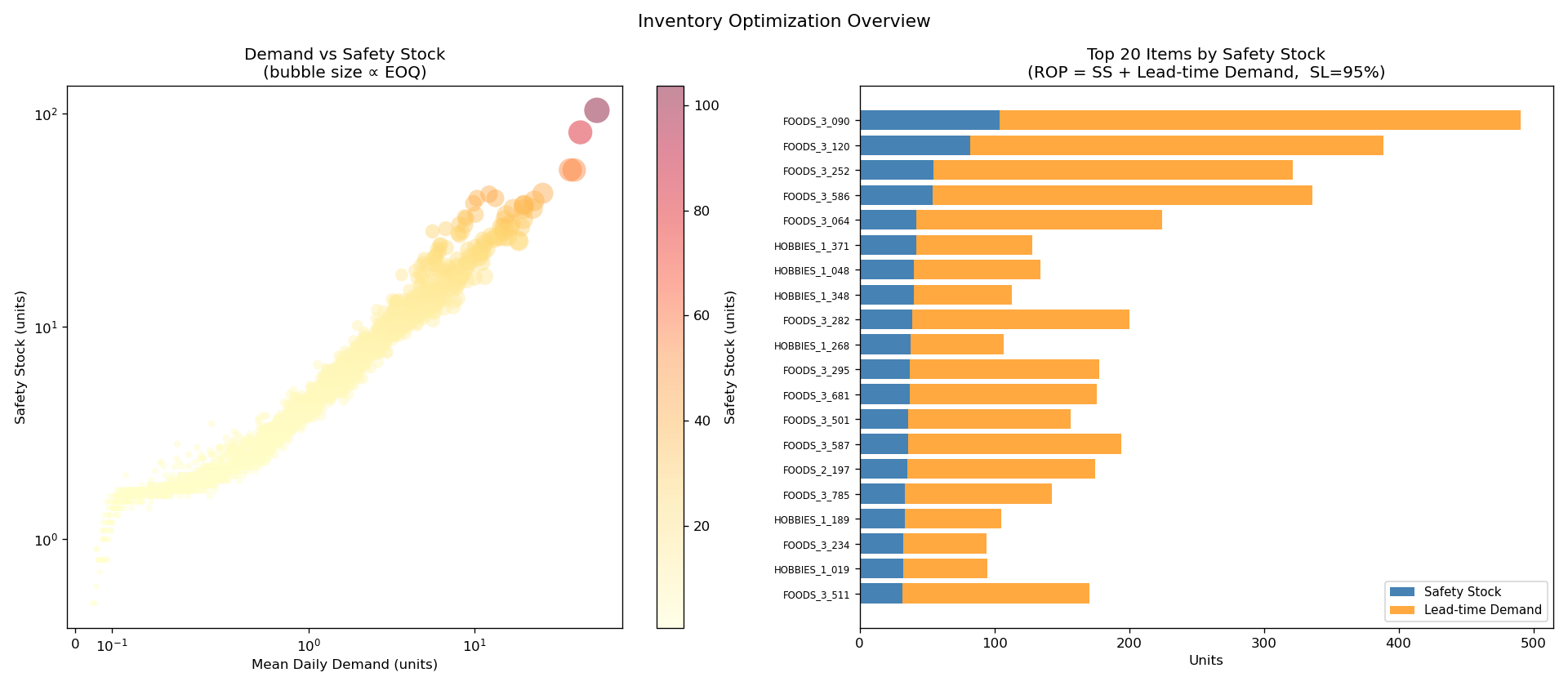
Example: Inventory Response

POST /inventory
{ "store": "CA_1", "item_id": "FOODS_1_001_CA_1_evaluation",
  "lead_time": 7, "service_level": 0.95 }

{
  "mean_daily_demand":  0.861,
  "demand_std_daily":   0.902,
  "lead_time_demand":   6.02,
  "safety_stock":        3.9,   ← hold this much buffer
  "reorder_point":       9.9,   ← order when stock hits this
  "eoq":                396.3,  ← order this many units
  "days_of_supply_ss":   4.6
}

Tech Stack

Data Processing

pandas, numpy, pyarrow, fastparquet

ML / Forecasting

LightGBM, statsmodels (ARIMA), Prophet, scikit-learn
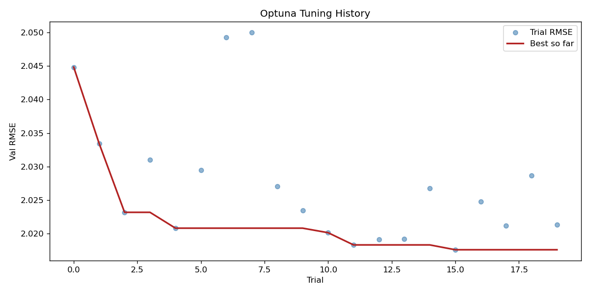
Optimization

Optuna (TPE sampler), 20-trial Bayesian HPO

Visualization

matplotlib, seaborn, plotly

API / Serving

FastAPI, uvicorn, Pydantic v2, TTL in-process cache

Dashboard

Streamlit (5-tab interactive app with live parameter sliders)

Seven-phase pipeline, end to end

1

Ingestion + EDA

Melt 5.9M rows from wide to long, merge calendar + prices, dtype optimization (categoricals + float32), 5 diagnostic plots.

2

LightGBM Global Model

Tweedie regression on all 3,049 series simultaneously. Lag, rolling, price, and calendar features. RMSE −29% vs Naive Seasonal.

3

Optuna Hyperparameter Optimization

20 TPE trials across 7 hyperparameters. Best params saved to JSON and reused in downstream phases.

4

Quantile Models (P10 / P50 / P90)

Three separate LightGBM models with pinball loss. 80% interval coverage: 83.4%. Quantile spread reused as volatility estimate in Phase 6.

5

Recursive 28-Day Forecast

Lag/rolling feature rollover loop. 28 sequential predictions per item. WRMSSE 0.911 (recursive) vs 0.877 (one-step) — only 3.9% degradation from compounding.

6

Inventory Optimization

Safety stock, reorder point, EOQ per item. Fully vectorized pandas — all 3,049 items in under 1 second. Configurable lead time, service level, and cost parameters.

7

Walk-forward Validation

4 rolling-origin windows (Feb–May 2016), full model retrain at each origin. RMSE CV = 3.1% — stable. 27–30% reduction vs baseline across all windows.